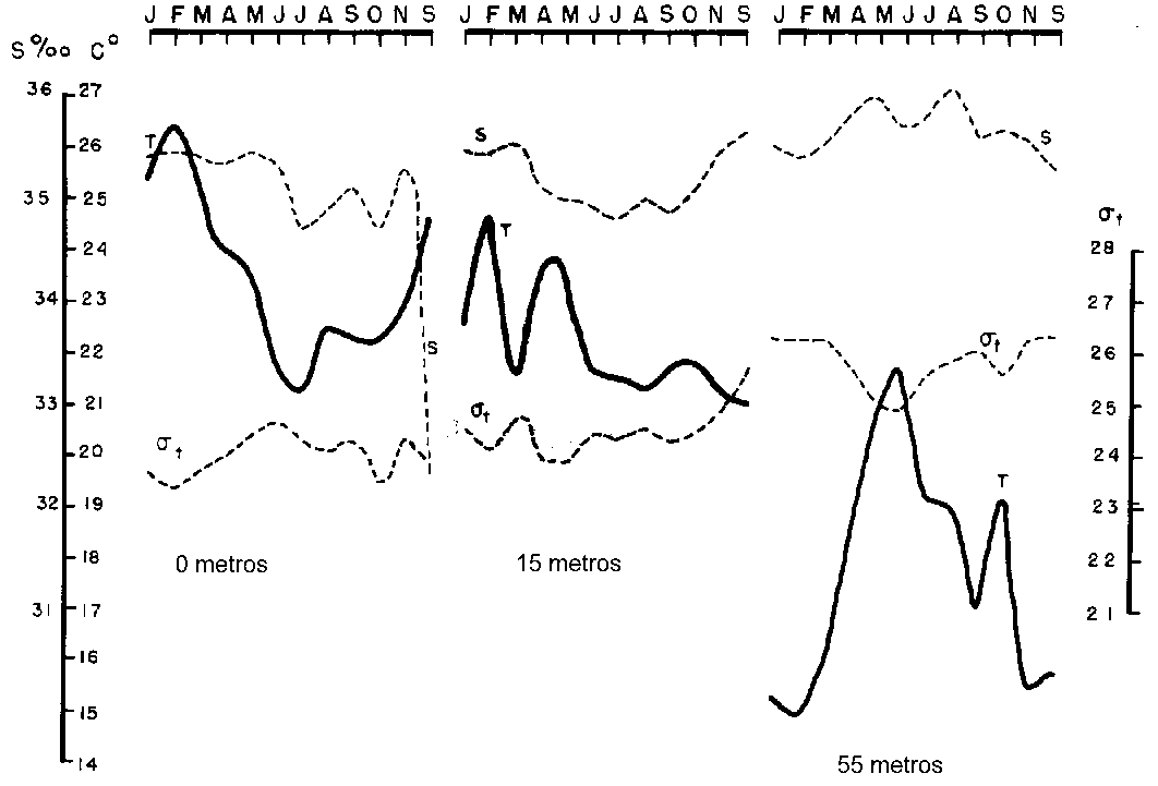
Figure 1 .– Mean seasonal temperature values , salinity and density at 0m 15m and 55m depth in the continental shelf of the south- eastern region in front of the city of Santos, SP, from (MESQUITA ,1969).
Afranio Rubens de Mesquita
E-mail ardmesqu@usp.br
www.mares.io.usp.br
January 2002
ABSTRACT
This work shows some aspects on the main characteristics of the hourly sea level, the daily sea level, the seasonal sea level and long term relative sea level along the Brazilian coast.
Key Words:
Brazilian Coast, Sea Level, Hourly, Daily,Seasonal, Long Term
1- INTRODUCTION
First measurements for fixing the datum for the mean sea level of the harbour of Rio de Janeiro were taken in 1831 as a series of one year length. The record is kept presently in the Museum of the “Diretoria de Hidrografia e Navegação” of the Brazilian Navy. Other measurements for tidal sea level keeping started to be taken by Federal organisms as “ Instituto Nacional de Pesquisas Hidroviárias” of the Ministry of Transport, since 1905 in various ports along the Brazilian coast, starting in different years, from the port of Belém in the extreme North to the port of Rio Grande in the extreme South of the coast and are now days poorly kept in the archives of that Institute.
It was only after the participation in the International Geophysical Year in 1958 that measuring the sea level acquired scientific flavour and moved researchers of the Institute of Oceanography of the University of São Paulo. Permanent tide gauges (registering instruments of the sea level Measurements via a buoy and a clock machinery) of the cities of Ubatuba and Cananeia were installed in 1967 and 1954, respectively. From these measurements emerged the first contributions on the sea level of the estuarine region of Cananeia, MINIUSSI (1958) and on the relationship of the sea level with the meteorological and sea water variables, JOHANESSEN, MIRANDA AND MINIUSSI, (1967) of Cananeia.
Harmonic studies of sea level for tides started in the beginning of the century in the “Observatorio Nacional do Rio de Janeiro” followed by tidal predictions performed with a Kelvin “tidal predictor” machine. ALIX LEMOS (1928).
The work of doing these analyses and predictions were passed to the “Diretoria de Hidrografia e Navegação” in 1964 (DHN, 1996), after the developments in the analysis there (FRANCO, 1968). Tidal constituents were determined from the measurements (periodical components of tides whose amplitudes and phases can be put into correspondence to the periodical motions of the Sun and Moon relative to a reference system fixed on the Earth) for the city of Cananeia (FRANCO AND ROCK 1972).
In response to an increasing interest of the community to the different aspects of the sea level along the Brazilian coast, MESQUITA AND HARARI (1983) produced the first report on tides and the tide gauges of Cananeia and Ubatuba, this can be called the local first period, of the scientific knowledge of the phenomenon of tides in the south-eastern coast and perhaps in the entire coast of Brazil.
Concomitantly, EMILSON (1961), (Physical Oceanography) first described the water masses of thesouth eastern part of the coast , MIRANDA (1970) produced the first calculation of the geostrophic currents of the same region, MAGLIOCCA Et Al (1979) first described the oxygen and nutrients distribution (Chemical Oceanography), TEIXEIRA, (1973) described for the first time the primary production of the waters and more recently AIDAR ARAGÃO (1980) (Biological Oceanography).
The seasonal variations of the Coastal Water analysed by MESQUITA (1969,1974) led to the identification of the phenomenon of “seasonal thermal inversion” that is typical of the region, as the Tropical Water and the Subtropical Water alternatively occupy the area seasonally. This produced in the layers below the thermocline, (region of the profile of temperature, near to the surface that suffers great vertical variation of the thermal values due to daily and seasonal variation of solar radiation) higher temperatures, during the winter months, and low temperatures, during the summer months. Figure 2.
Figure 1 .– Mean seasonal temperature values , salinity and density at 0m 15m and 55m depth in the continental shelf of the south- eastern region in front of the city of Santos, SP, from (MESQUITA ,1969).
This alternation is more intense specially in the coastal region near to Cabo Frio (RJ), where it was discovered also the phenomenon of "Coastal Upwelling", SILVA (1968) (oceanographic phenomenon by which the waters of the bottom layers come to the sea surface fertilising the oceanic region where it occurs).
2 -– SEA- LEVEL
The sea- level is amongst the measurements of the sea the one that synthesises the influences of various oceanic processes that include the effects due to marine currents, effects due to the field of mass , density, meteorological effects due to radiation, precipitation, evaporation, pressure, wind force and direction, effects due to the Earth’s geopotential , the geoid ( surface that has the same value of the acceleration of gravity), effects relative to the oceanic boundaries, effects due to the rotation of the Earth, as well as the effects of the tidal forcing due to the astronomical nature of the tides.
The last effect corresponds to the response of the ocean to the “Tide Generating Potential”, function written from the Universal Law of Gravitation of Newton, in terms of the rotation round common centre of masses and orbit parameters of the Earth, Sun and Moon, that allows the calculation of the gravitational and inertial forces that produce the Earth’s and Oceanic tides.
3 - HOURLY SEA LEVEL
The effects relative to the hourly variation of the meteorological parameters in the south eastern region may be seen in Figure 2, which shows the hourly sea level variation in Cananeia, during an occasion of a severe storm surge that covered the entire area. On the 25th of December of 1979 to the 5th of January 1980, simultaneous measurements of wind force and direction were recorded that are shown in Figure 3 in their north, south and east, west components. The wind directions were made the same as those of the currents, i.e., to where the winds go and not to what is usual in meteorology, from where the winds come.
The fluctuation of direction and wind force, associated with a pronounced variation of atmospheric pressure due the passage of an atmospheric “cold front, that occurred in an occasion of a sizygy ( the instant of the highest tide that occurs during Full and New Moon) produced a hourly variation of the tidal sea level of about 2 meters, and a daily variation of about 70 cm that caused a devastating effect, as the coastal cities of the entire South eastern area were invaded by the sea.
4 - The Daily Sea Level
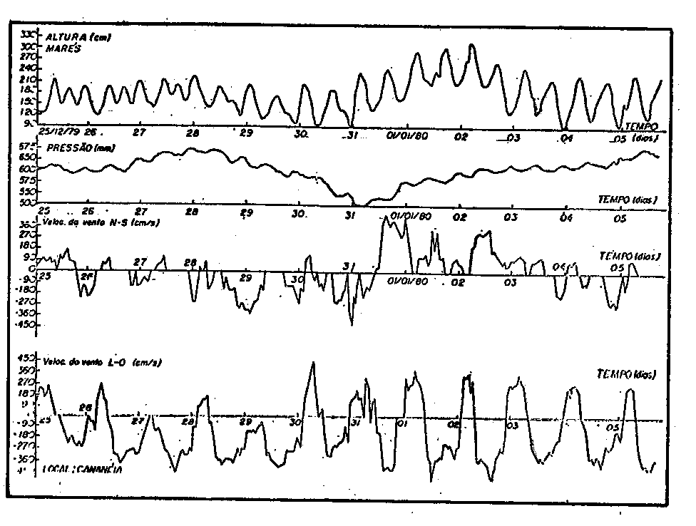
Figure 2.
Simultaneous records of hourlyatmospheric pressure, direction and wind
force (N-S; E-W) and the sea level recorded at the Research Station João
de Paiva Carvalho of Cananeia, during the 25 of December of 1979 to 6 of
January of 1980, from. (MESQUITA, ET AL 1989).
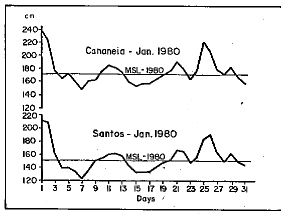
Figure 3 . Daily mean sea level variation of the cities of Cananeia and Santos during the period of 1st to 31st of 1980, from (FRANCO AND MESQUITA, 1986).
The mean
daily sea level (mean of the daily values of
the sea recorded during the period of 24 hours) of the same time interval
for the cities of Santos and Cananeia is shown in Fig. 3 and Figure 4,
the sea levels recorded in a different time interval of ports of Paranagua
and Cananeia. As can be observed the curves indicate that the variation
of the daily sea levels are highly correlated and are similar all along
the South-eastern coast.
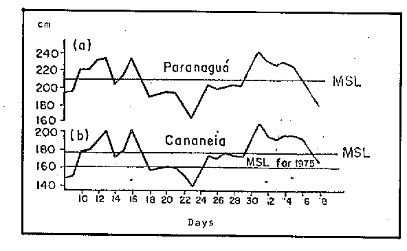
Figure 4. Daily sea levels of Cananeia and Paranagua. MSL stands for Mean Sea Level, from (FRANCO AND MESQUITA, 1986).
It may also be observed that pronounced deviation from the sea- level mean occurs frequently in the South-eastern coast without producing similar sea invasion of the coast, as occurred in 1st to 2d of January of 1980. With predictions that values of long term sea level rise that may reach 50 cm/century, however, even these minor variations of the daily mean sea level may frequently produce the invasion of the cities of the coast in not too far way distant future.
5 - THE SEASONAL SEA LEVEL
The first effort in the understanding the sea level seasonal variation (mean of the mean daily sea- levels recorded in the period of one month during all months of the year) of the city of Cananeia is shown in JOHANESSEN ET AL. (1967) Figure 5, in which they describe the relation with the meteorological variables as solar radiation, atmospheric pressure, wind force and direction, atmospheric precipitation, air temperature and sea temperature.
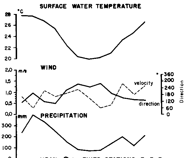
Figure 5 ; Upper part
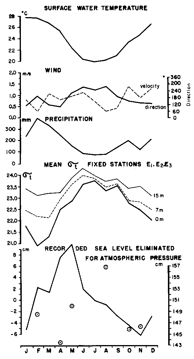
Figure 5 . Seasonal variations of, sea temperature from three stations on the near shelf coast, air temperature, atmospheric pressure, solar radiation and sea level in the research station João Paiva de Carvalho of Cananeia, SP during the year 1964, from (JOHANESSEN ET AL, 1967).
The amplitude
of the seasonal variation in the south eastern region is about 15 cm with
a secondary maxima in February caused by intense solar radiation and high
atmospheric precipitation and maxima in May that is interpreted by MESQUITA
HARARI AND FRANÇA (1995) as due to the steric variation (variation
of the sea water volume by effects due to temperature of the water making
the increase of the sea level) , of the sea level caused by the occurrence
in the South eastern region a greater volume of warm waters of the Brazil
Current that predominates in the area until the months of August to September.
Low values of
the seasonal sea level occurs in September, which after an increase in
November decrease in December to January, in consequence of the dominance
in the area of the colder Sub Tropical Water in the entire region. The
alternation of warmer waters in the winter months and colder waters during
the summer months gives rise in the region to the phenomenon of seasonal
thermal inversion, Figure 1. (MESQUITA, 1969,1974,1994).
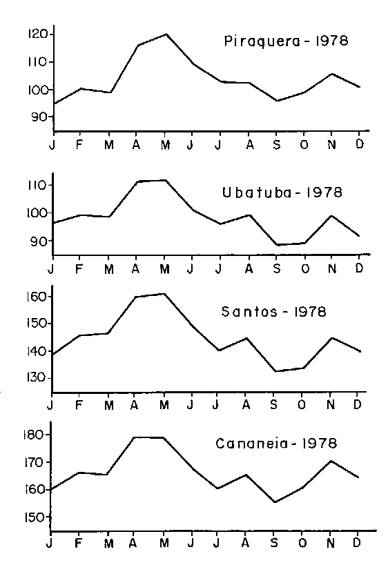
Figure 6. Seasonal sea level variation for the ports of Piraquera, Ubatuba, Santos and Cananeia in the year 1978 from (FRANCO AND MESQUITA, 1986).
Similar variability of the seasonal sea level is exhibited in the ports of Piraquera, Ubatuba , Santos and Cananeia in 1978 as shown in Figure 7. Similar variability is shown in all the Brazilian coast for the ports of Imbituba, Salvador, Recife, but differently by the port of Belém as shown in Fig 8. MESQUITA, FRANCO AND HARARI, (1987), from ten years measurements taken by the US Coastal and Geodetic Survey.
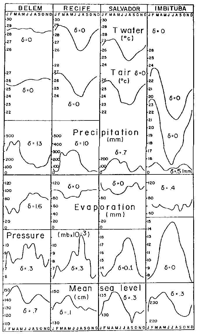
Figure 7 . Seasonal sea level variation of ports of Belem, Recife, Salvador and Imbituba (cm), air temperature,( C), sea temperature (C) , atmospheric pressure (mbar), precipitation and evaporation (mm) from 1953 to 1962; is the difference between the “Fourier fit” and the measurements along the Brazilian coast, from (MESQUITA, FRANCO AND HARARI, 1987).
The monthly sea level of Belem has two peaks, one in March/April and other September/October, that are probably due to the different regional river flow regimes of the northern and southern tributaries of the Amazon river. Ports of Recife, Salvador and Imbituba have similar variability as the Cananeia´s shown in Figs 6 and 7 with a secondary peak in February a maximum in April /May and lower values from August/September/October. Seasonal ranges are greater in Belem (20 cm) and smaller in Imbituba (10 cm).
6 - LONG TERM SEA LEVEL VARIATION
The long term sea- level also variation has a trend of astronomical origin. As the seasonal variation, for example, they are also excited by precise deterministic astronomical variations. The seasons in the South eastern region are astronomically determined by orbit compositions of the motion of the Earth around the Sun that produce the Summer and Winter Solstices (positions occupied by the Sun in the Southern hemisphere and in the Northern hemisphere during each year) exactly on 21st December and 21st of June.
The South-eastern Shelf responds to these compositions, said to be deterministic, (the one, one has almost absolute certainty) with maximum seasonal values of temperature of the sea water in Santos platform, with a turbulent delay of about one month later and with an uncertainty of its occurrence of one day, (MESQUITA AND HARARI, 1977). The recordings of this response, called random , or “turbulent”, are defined as “stochastic process” or “non linear process”, meaning in this case that the ocean of the south-eastern region responds “non linearly” to the deterministic astronomical action, fact which is also true all over the oceans.
The more one tries to determine with accuracy the thermal values of the sea water in the seasonal scale, bearing in mind the deterministic action that produce them, the more it is impossible to predict them with the same exactness. The same is true for the occurrence of the monthly thermal values, due to the unavoidable uncertainty inherent to the “stochastic processes” temperature of the sea water in the South eastern region. That is also what happens to the seasonal values of the mean sea level. They have their maximum (and minimum values) determined deterministically by summer and winter solstices position of the Earth around the Sun, but they actually only happen about a month later in Jan-Feb, (Jul-Aug) in the region. This is not actually quite followed by south-eastern waters in Figure 7 due to the “turbulent”, or nearly “random” influences on the mean sea level of the alternate occupation of the area by the Tropical and Sub Tropical waters as already pointed out.
A similar characteristic of uncertainty, one may admit, is attached to the interdecadal and decadal variations of the sea level recently identified in the region a by MESQUITA, HARARI AND FRANÇA, (1995,1996). Figure 8 shows the spectral distribution of the variabilities of the seasonal sea level of Cananeia. The spectral bands contain bands determined with a 95% confidence intervals that are centred in peaks exhibiting periodicities of 22 years (amplitude, 11 cm), 13 years (11 cm), 3.3 years (10cm) and 2.1 years (10cm ), that are excited by the variability of the ocean-atmosphere stochastic processes called ENSO (El Niño and Southern Oscillation) which themselves may have also some delayed relation with the variability of solar spots (MORETTIN ET AL. 1993).
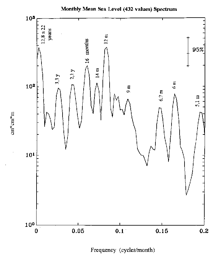
Figure 8 . Spectrum
of the oscillations of the relative sea level of Cananeia in the period
of 1954 to 1995, from (MESQUITA, HARARI AND FRANÇA, 1996).
In the spectrum are also identified spectral bands related to the stochastic processes of the long term sea level values of the South eastern region, as related to the Chandler Wobble (rotational of the Earth’s polar axis) of about 14 (10cm) and 16 months,(11cm) the band of 5 months(5cm) that probably are related to the Planetary waves ( waves generated by the moving field of mass and the Earth’s rotation) and the well known annual and semi-annual bands of the sea level.
Variabilities linked to the almost periodical astronomical forcing as the Earth’s declivity (inclination of the Earth’s North-South axis relative to its orbital plane around the Sun , the ecliptic) ; the precession of the equinox (position relative to the fixed stars of the days of the year , 21 of March and 23 of September, in which the nights and the days have equal duration) due to the rotation of the ecliptic and the variation of the Earth’s eccentricity (indices that measures how much the elliptic orbit is different from a circular orbit) are the causes of the stochastic processes of the almost periodical oscillations of the increase of polar ice and consequent diminishing of the mean sea level called glaciations.
Most of
the present records of tides are nearly long enough to identify some influence
of the precession of the equinox identified by the analysis of the tides.
The others glacial periodicities, however, can only be recorded in long
series, built from sediment cores (longsample
of sediments obtained with tubes that are forced into the bottom of the
ocean) from the oceans. Recorded series as long as 250.000 years have been
so far produced showing the almost periodical sea level variation during
the glacial periods, (EMERY & EMERY, 1980). Marks of the glaciation
in the south eastern region with the oceanographic evidences are shown
in FURTADO ET AL. (1996), and a summary of the variabilities, known as
of MILANKOVITCH , are reviewed in MESQUITA (1994, 1998).
7 - LONG TERM SEA-LEVEL VARIATIONS DUE TO GLOBAL WARMING”
Global Warming sea-level variations have recently been recorded all over the world´s continental borders. They differ from the long term variability of the sea level associated with the glaciations, as they became apparent from the beginning of this century till now and are characterised by an increase of sea level rate, as compared to the ones recorded before, (one to two mm/year).
As the world mean rate of open ocean sediment deposition in the bottom of the ocean, less than 1mm/year, HAYS ET ALL.(1976), TESSLER (2001), one may be inclined to attribute rates of about 4 mm/year, of the realtive sea level heights, as determined in the Brazilian coastal borders and from recent oceanic measurements of Altimetry, the distance of the satellite to the sea surface measured by the time delay between the emission and reception of a radar signal, of the Equatorial Atlantic (FRANÇA, 2000), as caused mainly, by extra global warming gases, (CO2, NH4, Water Vapour and others) expelled to the atmosphere, as a result of the increasing human activity.
The rate of variation
of the relative mean sea level has been recorded in the south-eastern region
since 1954, through the calculation of the inclination of the curves representing
the series plots of several ports of the area. The variability of the relative
sea level of the area and others in Brazilian coast are shown in Figure
9. As can be seen, not only the south-eastern coast but all Brazilian ports
are experiencing an increase of the relative sea level heights, level of
the sea obtained by tide gauges that are locked and fixed in the Earth’s
surface and it is impossible to determine if the ocean’s volume
is increasing, or if the land is sinking from these measurements only,
of nearly 4 mm/year or about 50 cm / century.
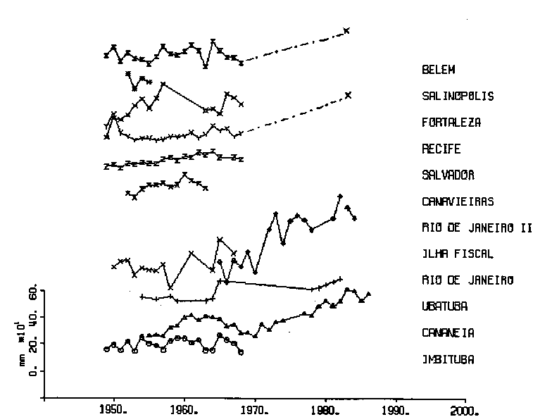
Figure 9. Series of annual values of the relative mean sea level (cm), of Brazilian ports of Belém, Recife, Fortaleza, Salvador,....,and Imbituba, from (FRANÇA, 1995).
Estimates of the global absolute sea level obtained via altimetry, however, are yet not definite (WOODWORTH , 1997) and evidences from geological studies of the local coast, as in MARTIN ET AL. (1987), as well the estimates based on all the series of the world’s ports from all continents including the poles , (MESQUITA, 1994) and the evidences of CHAO (1996), on the Milankovitch cycle in present days measurements are arguments that apparently oppose those figures. There is also evidence that the Brazilian coast may be sinking (MESQUITA, 1998), making the question of what is the main cause of the rate of increase, a rather controversial one.
To contribute the solution of these raised questions, collaboration is presently under way, with the Polytechnic School and the Institute o Astronomy and Geophysics of this University, the obtainement of measurements of GPS (Global Positioning System), (measurements of positioning on the surface of Earth by satellite, of great accuracy) and absolute gravimetry ( accurate absolute measurements of the acceleration of gravity) in the research Station João de Paiva Carvalho of Cananeia.
With these measurements
one will be able to determine if the geoid, where the sea- level gauges
are fixed, is changing (gravimetry) and the vertical motion (GPS) of the
terrain. These measurements are considered absolute and may help to find
out the accurate answer to the present controversies due to the Global
Warming, heating of the Earth due to the imprisonment of Solar energy by
the extra amount of gases as CO2, NH4 and others, produced by humanity
in the latest 100 years approximately, along the Brazilian coast.
8- CONCLUSIONS
Harmonic studies of sea level for tides started in the beginning of the century in the “Observatorio Nacional do Rio de Janeiro” followed by tidal predictions performed with a Kelvin “tidal predictor” machine . From 1964 on the tidal Tables for the brazilian ports were produced and published by the Diretoria de Hidrogafia e Navegacao.
The University of Sao Paulo (created in 1934), installed, in the fifities, and still operates through its Institute of Oceanography the permanent stations for measurement of sea level in the Cities of Cananeia ( Lat 25 S ; Long 47.5 W ) and Ubatuba (Lat 23.3 S ; Long 45.7 W ), along the Paulista litoral.
The hourly/daily variability of the sea level due to the variability of the wind force and direction accompanied by the variation of atmospheric pressure related to the passages of the cold fronts may reach 2 meters and the daily values about 70 cm above mean sea level in the borders cities of the south-eastern coast.
The seasonal sea level variability is smaller in the southernmost ports as Imbituba (10cm) and greater in Belem (20 cm). Belem has two sea level seasonal peaks, one in March/April and other in September/October probably due to the Amazon river flow annual variability. They show peaks in February for ports situated in the East coast caused by intense solar radiation and precipitation and a maximum level in May, caused probably in the south-eastern region by the steric effect due to the occurrence of a greater volume of warmer sea water of the Brazil Current that remain until August-September.
In August-September-October occur the lowest levels of the seasonal sea level that after a small increase in November fall again during the months of December and January due to a greater volume of colder Sub-Tropical waters. This alternate predominance of water masses in the area gives rise to the phenomenon of “seasonal thermal inversion” that may eventually occur also in the entire east Brazilian coast .
The spectra of seasonal sea level values in south-eastern have spectral bands, determined with 95% confidence intervals, with peaks around 22, 13, 3.3, and 2.1 years that are supposed to be related to the El Niño/Southern oscillation of the Pacific (ENSO) and ultimately related to the variability of the solar spots and atmospheric precipitation in the north-east part of the country.
With the same statistical interval were also determined bands related to the 14 and 16 months periodicities of the “tide pole” the 12 months band (the annual tides, that is as strong as the 13 to 22 years Brazilian northeast draught bands) and the 5 months band of the planetary waves.
The long term sea level of the relative mean sea level indicate that in the Brazilian coast it is increasing at a rate of 4 mm/year or about 50 cm/ century. The most probable of its causes is the now days thenb extra global warming gases produced and emitted to the atmosphere.
9 - ACKNOWLEDGEMENTS
Special thanks are due to FINEP (Funds for Studies and Projects of the Presidency of the Republic of Brasil) and FAPESP (Foundation for Research Aid of the State of São Paulo).
10 - LITERATURE CITED
AIDAR - ARAGÃO, E . A., TEIXEIRA, C. AND VIEIRA, A H. (1980). Produção primária e concentração de clorofila a na costa brasileira ( Lat 22 31 ; Long 42 52 W). Bolm. Inst. oceanogr. Univ. S. Paulo. S.P. 29 (2) : 9 - 14.
BELFORT VIEIRA, J. D. 1942. As Marés , Observação Estudo e Previsão no Brasil. 169 paginas. Ver Biblioteca do Instituto Oceanográfico da Universidade de São Paulo.
CARTWRIGHT, D. E. (1999). Tides- A Scientific History. Cambridge University Press. Cambridge. UK.
CHAO B F. (1999). “Concrete” Testimony to Milankovitch Cycle in Earth’s Changing Obliquity. EOS, Trans. Am. Gophys. Union. Vol ( 77 ) . Number 44. : 433 .
DHN (Diretoria de hidrografia e Navegação) .1996. Tábua de Mares para 1997 .Min. mar. Rio de janeiro. Vol 34 : 1 - 196.
EMILSON I . (1961). The Shelf and coastal waters off southern Brazil. Bolm. Inst. oceanogr. , Univ. S Paulo. 11 ( 2 ) : 101 - 112.
IMBRIE, E, AND J. IMBRIE, N. (1980). Modelling climatic response to orbital variations. Science, 207:950-953.
FRANÇA C A S .(1995). O litoral Brasileiro - Estudos sobre o nível médio do mar. 1993. (Não publicado) Insti. oceanogr. Univ. S Paulo. (ver Biblioteca do IOUSP). 21p.
FRANÇA, C A de S. (2000). Contribuição ao Estudo da Variabilidade do Nível do Mar na Região Tropical Atlântica por Altimetria do Satélite TOPEX/POSEIDON e Modelagem Numérica. Tese de Doutorado. Instituto Oceanográfico da Universidade de São Paulo. 274p.
FRANCO, A S. (1968). The Munk - Cartwright method for prediciton of discrete observations. I H. Review . 42 (I).
FRANCO, A S AND ROCK, N J . (1972). The fast Fourier transform and its application to tidal oscillation. Bolm. Inst,. oceanogr.Univ. S. Paulo. SP.
FRANCO, A S DOS AND MESQUITA, A R DE. (1986).On the Practical use in Hydrography of Filtered daily values of mean sea level. Int. hidrg. Rev. Monaco. LXIII ( 2 ) : 133 - 141.
FURTADO,V.V., BONETTI, J.FILHO AND CONTI, L. A. (1996). Paleo River morfology and sea level Changes as the southern Brazilian continental Shelf. An. Acd. Bras. Ci., Vol 68. Supl. 1:163-170.
HAYS, J. D., IMBRIE, J. AND SHACKLETON, N. J. (1976). Variations in the Earth's Orbit: Pacemaker of the Ice Ages. Science. Vol 194. Number 4270 : 1121 - 1132.
JOHANNESSEN, O M., MIRANDA, L B. AND MINIUSSI, I. B. (1967). Preliminary study of seasonal sea level variation along the Southern part of Brazilian coast. Contrções Inst. oceanogr. Univ. S. Paulo, ser. Oceanogr. fis. (9) : 16 - 29.
LEMOS, A. (1928). Marés e Problemas Correlativos. Observatório (Astronômico) Nacional do Rio de Janeiro. RJ. 92p.
MAGLIOCCA A , MIRANDA L B DE AND SIGNORINNI, S. R. (1979). Physical and Chemical aspects of the transient stages of the upwelling at the southwest of Cabo Frio (Lat 23 S ; Long 42 W). Bolm. Inst. oceanogr. Univ. S. Paulo. Vol ( 28 ) , 2 : 37 - 46..
MARTIN, L., SUGUIO, K., FLEXOR, J. M. , DOMINGUES, J M L. AND BITENCOURT, A C M S. (1987) . Quaternary evolution of the Central part of the Brazilian coast. The role of the relative sea level variation and shore line drift. In Unesco Quaternary Coastal geology of West Africa and South America. UNESCO Reports in Marine Sciences n 43 : 97 - 145. Paris. France.
MESQUITA A R DE (1969) . Variações sazonais nas Águas Costeira. Brasil Lat 23. Diss. Mestr. Inst. oceanogr. Univ. S Paulo. SP. 78 p.
MESQUITA A R DE (1974) . Report on the seasonal variations of coastal Waters; Brazil (Lat 24 3 S). Relat. int. Inst. oceanogr. Univ. S Paulo. SP. (1) : 1 - 36.
MESQUITA A R DE AND HARARI J (1977). Variações sazonais em águas costeira: Brasil Lat 24 . Parte II. Bolm Inst. oceanogr. S Paulo, 26 : 339 - 365, 1977.
MESQUITA A R DE AND HARARI J (1983). Tides and Tide Gauges of Cananéia and Ubatuba. Relat. int. Inst. oceanogr. Univ. S. Paulo. SP. (11) : 1 - 14.
MESQUITA A R DE AND LEITE J B A (1986). Sobre a Variabilidade do Nível Médio do Mar na costa Sudeste do Brasil. Rev. bras. de Geofis. Vol ( 4 ) : 229 - 236.
MESQUITA A R DE., FRANCO A S. AND HARARI J. (1986). On mean sea level variation along the Brazilian coast I. Gephys. J. R astr. SOC. London Vol ( 87 ( 1 ) : 67 - 77.
MESQUITA A R DE AND FRANÇA C A S (1989). Tidal Statistics of Varadouro Channel as Inferred from Cananéia tidal Station.Academia de Ciencias do Estado de São Paulo. S Paulo. vol ( 2 ) : 242 - 254.
MESQUITA A R DE AND FRANÇA C A S (1991). On the transference method for the mean and extreme sea level values. Acad. ci. Est. S Paulo. S Paulo. SP. Vol ( 1 ) : 55 - 64.
MESQUITA A R DE (1994) .Variação do nível do mar de longo termo. Inst. est. Avanç. Univ. S Paulo. SP. Documentos - Série Ciências Ambientais.Vol ( 20 ) : 47 - 67.
MESQUITA A R DE , HARARI, J. AND FRANÇA C A S (1995) Interannual variability of tides and sea level at Cananéia , Brazil, from 1955 to 1990. Publcão esp. Inst. oceanogr. Univ. S Paulo. SP. (11) : 11 - 20.
MESQUITA A R DE , HARARI, J. AND FRANÇA C A S (1996). Global Change in the South Atlantic: Decadal and Intradecadal Scales. An. Acad. bras. Ci., Vol( 68 ) . Supl.1 : 117 - 128.
MESQUITA, A R De (1998). O programa IOUSP para o Global Changes : Origem e Contribuições. Apresentado no Seminário Ciência e Desenvolvimento Sustentável. Inst. est. Avaç. Univ. S. Paulo. SP. Volume único : 130-146.
MINIUSSI, I. C. (1958). Nível médio , nível de redução das sondagens e a variação anual do nível médio mensal do porto de Cananéia. Contrçõs Inst .oceanogr. , Univ. S Paulo, ser. Oceanogr. fis., (2) : 1 - 7.
MIRANDA, L B DE (1970). Flutuações da Corrente do Brasil e variações da distribuição horizontal da temperatura na região costeira entre Cabo de São Tomé e Ilha de São Sebastião em Janeiro e Fevereiro e Abril de 1970. Caderno de Ciencias da Terra, São Paulo, 3, parte 2 : 13 - 14.
MORETTIN, P A, TOLOY, C M, GAIT, N AND MESQUITA A R DE. (1993). Analysis of the Relationships between some natural phenomena: Atmospheric precipitation , mean sea level and sunspots. Rev. bras. Metorolol. 8 (1 ) : 11 - 21.
SILVA, P M C DA (1968). O fenômeno ressurgência na costa meridional brasileira. Publições Inst. pesq. Mar. Vol ( 24 ) : 1 - 31.
TESSLER, M. G (2001).Taxas de Sedimentação Holocênica na Plataforma Continental Sul do Estado de São Paulo. Tese de Livre Docência. Inst. oceanogr. Univ. S Paulo. SP. 155p
TEIXEIRA
C. (1973). Preliminary studies of primary production in the Ubatuba region
( Lat 23 30 S ; Long 45 06 W), Brazil. Bolm. Inst. oceanogr. Univ. S.,Paulo
SP. 22 : 40 - 58.